Video

Summary of the project

Crop farming in Minecraft can be quite a time consuming process: to get any significant benefit in the game, we have to first find suitable spots for the seeds to grow, and then physically go to each of those locations to plant them. Even if as a human user we spend a lot of time finding locations, they may not even be optimal planting positions, especially if the mechanics of minecraft farming aren't known. So to make the process quicker and easier we have made a tool that allows an AI to do the farming process for you and save more time for you to do whatever else you want to do in the game.

While farming in minecraft is quite intuitive, farming successfully and optimally is no easy task. There are countless blogs that can be found explaining to players about the greatly varying results based on a number of criteria. These include:

• Terrain: which block you place seeds on directly influences crop yield
• Proximity to water: the closer to a river/water, the faster crops grow
• Light: even if artificial, more light generally means a higher crop yield
• Material Additions: Materials like Bone Meal can help make crop yield faster

So, the final aim of this project was to create an agent such that, given a map and some farmable objects (wheat, pumpkin seeds etc), will plant the objects for the user in an optimal position on the map, based on the researched criteria above. We specifically thought AI algorithms are suited to this problem because, as explained in our approach and evaluation sections below, we can map this to a search style problem that can use genetic algorithms to progressively optimise our score function; completing this process of searching squares, scoring particular squares, and then selecting the best squares as a human user, especially with no knowledge of minecraft farming, would be very time consuming indeed.

Approaches

We will be using a Genetic Algorithm to solve this problem, which essentially involves mapping the problem to a graph search problem and following a procedure of breeding successful states to allow our seeds to converge onto an optimal location.

The graph in this case will be our map: each square is a node in our graph, with each graph node carrying some notion of a score. Optimal zones will carry the highest score, so our problem can be seen abstractly as locating the maximum points on a graph. Visually, it is something like this:

So essentially, there are areas that are "hot" (maxima in the graph- close to water for example) and "cold" (minima in the graph- dry dirt for example), which our algorithm must differentiate

Checkpoints

Baselines

Setup

To set the agent up with what it needs, we do the following:

• First, to create a test environment for our project, we generated a very simple world, which is essentially a square grid containing:
  1. A water square at (0,0)
  2. Dirt around the water from (-10,10) in the (x,z) directions
  This has the implication of creating hydrated water from (-4,4) by [AKA the "optimal" part of the map and where plants will grow fastest] and leaving the remaining dirt squares as dry, and non optimal/ unplantable.
• The agent is given a range of squares to plant in, which for our purposes, are any of the squares in (-10,10): the agent is successful if he puts a majority of the seeds in the hydrated square region at the end of the algorithm

Baseline 1

As stated in the status report, the absolute benchmark we have used for this project is a random agent. That is, an agent that follows a procedure like so:
Set size <- length of side of the map (assuming it is a square)
For i in N seeds
Generate (x,z) where x and z are in the range (-size, size)
Evaluate the N seed locations

Please see the status report for a mathematical breakdown of this method

Why was this method used as the baseline?

Firstly, it makes reasonable intuitive sense: for a player who has never played minecraft before and is asked to plant some seeds, it is reasonable to assume that they will essentially begin planting in random locations, trying to learn the rules of the game. Apart from that, it is also important to note:

• This needs virtually no startup data: all we need is the size of the map, and we can begin to get details about the benchmark we should be beating with our algorithm
• It generalizes incredibly well: we can get a benchmark for almost any map by use of this algorithm

The challenge is now to improve the accuracy

Baseline 2/ the MVP/ first test case

After studying genetic algorithms and how they function, we wanted to apply it to a very basic map, with mostly hard coded values binding closely to the current map, to see what kind of improvement we could get over our random algorithm. We ended up with the following procedure:

• We initialize 10 random seed locations, stored as (x,z) tuples [Y is implicitly the same as we do no digging]
• For 10 rounds, we:
  • score the current seed locations using our scoring function, which essentially measures distance to the nearest water block
  • take 5 "elite" seeds: that is, the best scoring seeds from the group. These 5 seeds automatically pass to the next round of seed locations
  • using the same 5 best seeds, generate 5 new children seeds by using their attributes. In this simple version of our algorithm, we essentially randomly take the x and z coordinate from either of the parents. This is a simple approach, but is quite effective is generating good results.
  • The 5 best seed locations are taken along with the new 5 children, ready for the next round. The worst 5 "die"
  • Randomly mutate one of the seed locations by adding a mutation vector, which for now, adds (x,z) to a seed location where x and z are both in the range of [-3,3]
• At the end of the generation of seed locations, we have a list of (x,z) pairs to place our seeds. We then plant these, and calculate how many were placed in the (-4,4) farmland section

This left us with an algorithm, currently usable only for the one map, that we could use to compare our genetic algorithm to our random agent with

This had the following properties:

• The algorithm was evaluated to be highly accurate (see the status report for more details on this benchmark). We were able to get our success rate to 92% (compared to roughly 30% for the random algorithm) which let us know we were at least on the right track.
• This model was very hard to maintain however: the details of where each of the block types (water, dirt etc) had to be manually fed in to the agent. The number of seeds to plant, as well as the number of rounds the agent would run for, were all hard coded.
• This led to the biggest of our concerns: overfitting of our current algorithm to our one particular map instance.

So now, for the final stretch of our project, we wanted to generalize our algorithm to work for any given map.

The Final Algorithm

• We initialize N random seed locations [N could be any integer value less than the map area], stored as (x,z) tuples [Y, aka depth, is implicitly the same as we do no digging]
• until convergence, we do:
  • score the current seed locations using our scoring function, which essentially measures distance to the nearest water block
  • take 50% of the seeds as "elite" seeds: that is, the best scoring seeds from the group. These 50% automatically pass to the next round of seed locations
  • using the same best seeds, generate the remaining required 50% new children seeds by using their attributes. For our final algorithm, we essentially randomly take the x and z coordinate from either of the parents. This is a simple approach, but is quite effective is generating good results.
  • The best half of the seed locations are taken along with the newly generated children, ready for the next round. The worst half "die"
  • We also randomly mutate one of the new seed locations by adding a mutation vector. The mutation vector is in the range of [x,z] => [-mapsize to mapsize, -mapsize to mapsize], with the range decreasing by 1 block every round. This continues for 5 rounds, meaning that we get large mutations in the beginning, used for map exploration, before cutting it off later in the process (under the assumption that a reasonable spot has been found in those 5 rounds)
• At the end of the generation of seed locations, we have a list of (x,z) pairs to place our seeds. We then plant these, and calculate how many were placed in the hydrated farmland section

So as you can see, key modifications to this algorithm now include:

• The number of seeds is generalized. This means we could experiment with different numbers of seeds to see how our algorithm would react.
• The convergence of the algorithm has now been defined, and is not simply defined to just stop at round 10. See below for an exact definition of what convergence means in our algorithm.
• Mutations have been set up to explore the map far more aggressively: we start with being able to mutate a seed anywhere in the map, then progressively decrease the range (by 1 unit on x and 1 unit on z) each round. After 5 rounds, exploration stops, and we attempt to converge on whatever the best points we have found are,

This modification to our algorithm base had the following hopeful properties:

• It would be reasonably accurate (better than random) for the maps we give to it
• It would not require us to manually specify where each block type was: instead, we would query the world for a JSON array corresponding to the block types at each position
• It would not overfit onto properties of our initial test map

What is convergence?

Convergence in our algorithm was a little harder to define: initially we believed that it would be enough to simply check to see if our score was beginning to balance out: that is, if the rate of change of the score had decreased below a threshold, we would stop.

This didn't turn out to be enough however: in many cases, this approach would work, but it turned out that in some cases, the score would wildly sometimes, especially if the seeds were already in an optimal postion, and the next round then moved a seed sub-optimally, causing it to rapidly decrease it's score, and then immediately increase rapidly the following round.

So instead, we played a game of averages with our scores every round. At each round, we would do the following:

• If we haven't gone 10 rounds yet, return
• Else, get the history of scores for the last 10 rounds
• Calculate the average of those 10 scores to get a mean score
• Now if in the last 10 scores, there have been 5 that have moved "significantly" away from the mean in the positive direction, then we keep going. Otherwise, we terminate, as the scores have failed to change significantly/ change positively in the last 10 rounds.
• Significantly is defined as being 3 points away from the mean

This method turned out to work remarkably well in terms of calling the algorithm to terminate when needed.

NOTE: an alternative we considered was to use a "Max score" property: aka calculate a maximum available score and check if the current score is near this. We decided against this approach, simply due to generalization. The above method is quite robust to changes in the number of seeds and change of map. However for the latter method, a max score would need to be manually recalculated for each map and number of seeds. We felt this was unnecessary to do, especially after testing showed the former algorithm to work quite well.

Evaluation

We will provide a comprehensive evaluation of our final genetic algorithm, testing by varying our parameters in the algorithm and maps that we run the algorithm on to test generalization.

Map 1: initial test map

This tests the map that has the features:

• A water square at (0,0)
• Dirt around the water from (-10,10) in the (x,z) directions

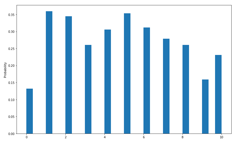
Chart 1: Accuracy Data

The above chart shows a histogram plot of 1000 runs of the algorithm on 10 seeds, with the y axis representing the number of times that that particular seed number was planted. As you can see, for this original test map, the generalised algorithm does quite well, with the dominating probability/ frequency being 10 seeds out of 10 planted.

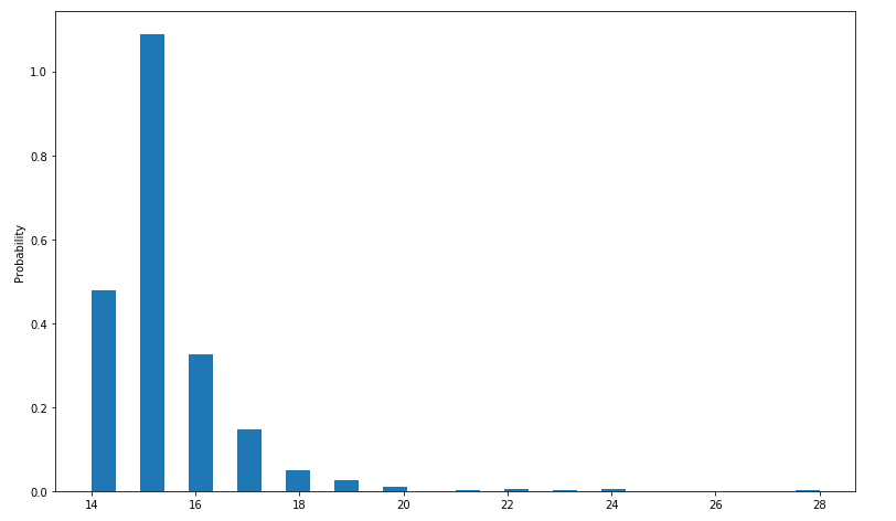
Chart 2: Convergence Data

Another interesting aspect we wanted to investigate was a profiling of when the algorithm terminates. The above chart shows the frequency of rounds when the algorithm terminates. We see an interesting rough normal distribution appearing, centered around 19 as the rough mean. this provides us valuable information about how reliably our algorithm converges, aka, whether there is some kind of pattern or whether it "stumbles" onto a solution. In this case, we see that the algorithm has quite a defined convergence pattern, and indeed if we were to have some finite number of rounds to execute in, we could start to estimate our success rates with such a graph.

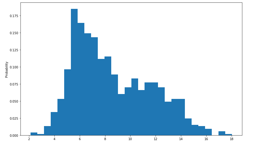
Chart 3: Euclidean Distance between seeds

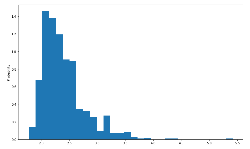
Placing crops in an organized manner close to each other is an important aspect of minecraft farming. We wanted to run a test of average (Euclidean) distance for a point to the rest of the points on a graph/ map we knew was successful to use as a baseline for testing whether map size/layout has an impact on proximity of plants to one another. The initial test results are summarized in a histogram above, which defines ranges for the Euclidean distance and then buckets the results from 1000 runs into their corresponding frequencies.

We see that, for our ideal test map, the most common global distances are between 2 and 2.5 blocks. We will use this as a reference point for future maps.

Varying the seeds

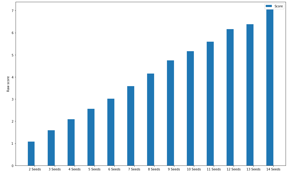
Chart 4: Accuracy Data with varying seeds

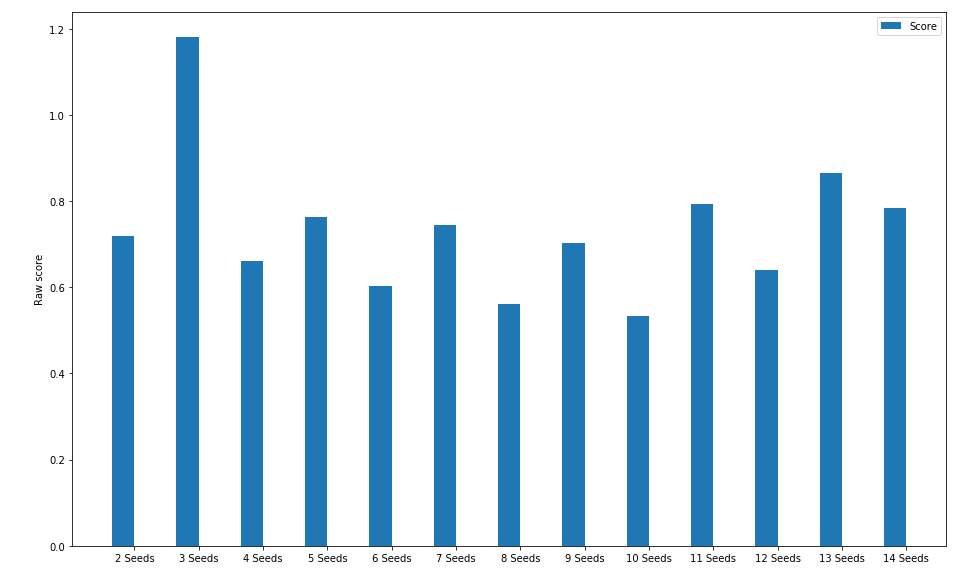
This time, we repeated the accuracy test (how many seeds from the available were planted) but this time, the above chart essentially shows (over 1000 runs for each number of seeds) how many seeds we actually lost.

Very interestingly, it seems that in this map, the number of seeds that were misplanted has no correlation with the number of seeds available: that is, no matter how many seeds you start off with, you'll always get roughly one of them planted in a non optimal area

This can be explained with the following:

• We found earlier that our accuracy was above 90%. So for all values of number of seeds, it makes sense that very few are lost
• There is an interesting up/down movement occurring in the chart, which represents even numbers of seeds are more successful than odd numbers of seeds. This is because, in the even number of seeds, a clear line between 50% children and 50% elite seeds can be drawn. The same cannot be said for odd numbers of seeds: so we must draw (n+1) children from only n seeds. This small bias means there is less variation in the offspring we produce, and so the odd numbers of seeds automatically have a lower success rate.

Chart 5: Convergence Data with varying number of seeds

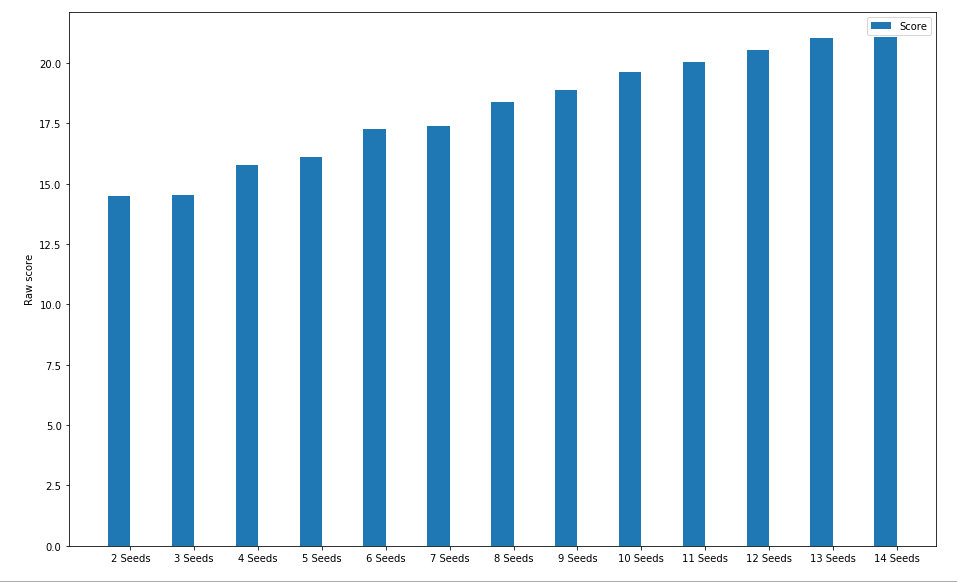
This time, we repeated the convergence test (how many rounds until reasonable confidence that the optimal solution has been found) but this time, the above chart essentially shows (over 1000 runs for each number of seeds) how many rounds on average it took until we artificially broke out of our round loop, under the confidence that we have the right solution.

As we expected, the more seeds we have, the more rounds it takes to be confident that all of those seeds form in some kind of (near) optimal position.

Generalizing our current solution

Now, we aim to take our generalized algorithm (after testing on our base map) and try it on different maps, to see if we managed to succeed to make it general for different kinds of structures/ challenges.

Map 2: Surrounding water map

This map is now flipped: rather than focusing on one water square that hydrates a central area, we wanted to see how our algorithm performs when the water is Surrounding the territory.

We made a map which looks something like this:

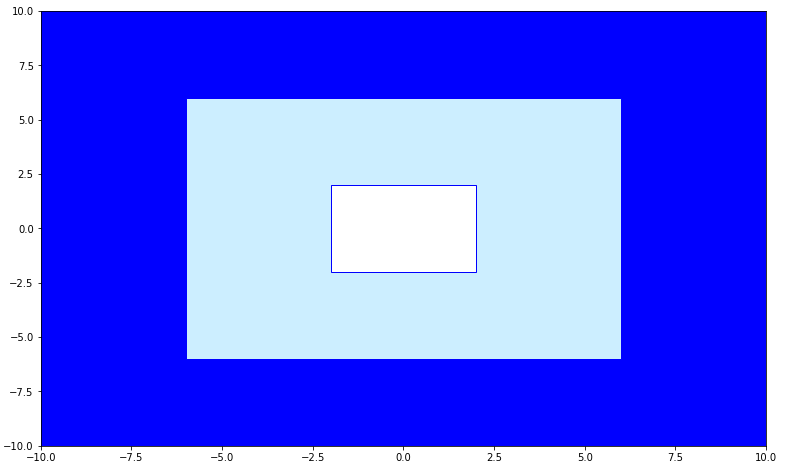
(White is rock, light blue is plantable area, dark blue is water)

The map is the same size as the initial map above, but this time, water has been added to surround the farmland rather than just be a central point. We hope to issue this to the agent as a challenge to see how it will deal with multiple optimum points.

We will now use the same evaluation metrics on this map to compare to the initial map

Chart 1: Accuracy Data

The above chart shows a histogram plot of 1000 runs of the algorithm on 10 seeds, with the y axis representing the number of times that that particular seed number was planted.

As you can see, for this map, the accuracy has dropped on this map: while still better than using a random agent, there is a noticeable decrease. The histogram shows this quite nicely by how spread out the bars are compared to the first chart, that is, there is much more uncertainty now about how many seeds an agent will correctly plant compared to our small initial map. We expect this inaccuracy to stem from the fact that water now surrounds the entire planting area; this means that now, when two seed locations are crossed over, there is a potential that the two selected seed co-ordinates are at opposite ends of the map. This in turn means that if we take one co-ordinate from one, and one from the other, a seed could end up in the middle of the rock at the center of the map. To prevent something like this in the future, we could theoretically have used a less strict convergence algorithm, which would have let more potential mutations be tried out, and so more chance of two seeds landing next to each other would have been explored.

Chart 2: Convergence Data

As you can see from this chart, the convergence hasn't significantly changed for this map. Indeed, we wouldn't exactly expect it to either: the maps were the same size, so the agent doesn't have to necessarily decide on any more squares than it had in the initial map.

Chart 3: Euclidean Distance between seeds

The test results are again summarised in a histogram above, which defines ranges for the Euclidean distance and then buckets the results from 1000 runs into their corresponding frequencies.

The histogram has shifted in the positive direction and spread itself out: so now we have more variance in where seeds land and how many land in a particular region. This of course makes sense: the optimum region now is quite large so seeds have a lot more freedom of where they could select their final location.

Varying the seeds

Chart 4: Accuracy Data with varying seeds

Again, the accuracy is better than what a random agent would perform like, but this time compared to our original test map, the number of seeds misplanted linearly rises with the number of seeds. This is because this time, the planting rate isn't (almost) perfect like on our initial training map, and has an error rate which is quite high: so as the number of seeds rises, so does the number of misplanted seeds.

It is interesting to see however that the error rate doesn't change with the number of seeds, which can be seen because of the linearly rising pattern of the graph.

Chart 5: Convergence Data with varying number of seeds

Again, the above chart essentially shows (over 1000 runs for each number of seeds) how many rounds on average it took until we artificially broke out of our round loop, under the confidence that we have the right solution.

We see that the number of rounds needed to accept the current planting co-ordinates and stop searching is roughly independent of the number of seeds, or at least rises very slowly with number of seeds.

Summary/ comparison of results

So from these results we can mostly take that, while our algorithm still does perform better than a random agent would on the same map, it is quite inaccurate compared to our initial map. This suggests there is some deal of overfitting taking place that makes our algorithm unable to generalize fully when taken into a different style of map, with water surrounding the farmland rather than there being one central point of water.

Map 3: Large map, corner water spot

This time, we wanted to see how our algorithm would perform on a very large map. We created a map which was 50x50 in size, and wanted to see whether our algorithm would manage such a large scale map/ find the hydrated zone by use of the mutations.

Results

For brevity, we will not be including the full run down of all charts, since the results can be easily explained

We found that, for maps much greater than 20x20, the algorithm just wasn't able to find the hydrated farmland section. The reason is mostly the map exploration side of the algorithm: at the moment, the algorithm does not invest a lot in finding new sections of the map, meaning that unless it gets lucky at the start with a seed generation in the hydrated zone, it most likely won't find the needed optimal section.

Overall Summary

To quickly conclude the project report, I hope the reader has seen that we have successfully made a genetic algorithm that can solve the problem of optimally planting seeds for basic maps, of a resonably small size.

In the future, would this project have continued, we would have a lot of scope to improve the algorithm to make it work far more generally than it does now. The most important changes we could make would most likely be to the score function, to incorporate additional minecraft farming parameters such as torches, or to the mutation algorithm, so that the algorithm would explore maps more thoroughly, so that it could deal with larger map sizes.

Overall we hope you have enjoyed reading about the project and thank the professor and TAs for their continued support and education throughout the quarter.

References

Specific software technologies

We used matplotlib to generate all figures used throughout this webpage. Matplotlib is a plotting library for the Python programming language, which we used together with jupyter notebook, an open-source web application that allows you to create and share documents that contain live code, to generate our figures and test the output we were getting

References to both are below

Jupyter notebook

Visit here to read more

Matplotlib

Visit here to read more

Referenes to resources on Genetic Algorithms

Below is a list of resources we found useful when researching Genetic Algorithms

Matlab Article

This resource demonstrates how a genetic algorithm is used to find minimum points on a graph

A nice breakdown is given of the seperate stages of the genetic algorithm and how you can actually code up a solution by yourself

Visit here to see the article

Video Demonstration

The below video shows a nice visual animation on how genetic algorithms repeatedly take the best performing samples from the "gene pool" to eventually converge on a population that each finds itself on some optimal point.

See the video on youtube here

Washington University

This gives a brief insight into how genetic algorithms came about and a general overview of implementation

See it here

Wiki page

Gives a few good examples of genetic algorithms

See it here